Improve Forecast Accuracy with TimeGPT

In this notebook, we demonstrate how to use TimeGPT for forecasting and explore three common strategies to enhance forecast accuracy. We use the hourly electricity price data from Germany as our example dataset. Before running the notebook, please initiate a NixtlaClient object with your api_key in the code snippet below.

Result Summary

Steps	Description	MAE	MAE Improvement (%)	RMSE	RMSE Improvement (%)
0	Zero-Shot TimeGPT	18.5	N/A	20.0	N/A
1	Add Fine-Tuning Steps	11.5	38%	12.6	37%
2	Adjust Fine-Tuning Loss	9.6	48%	11.0	45%
3	Fine-tune more parameters	9.0	51%	11.3	44%
4	Add Exogenous Variables	4.6	75%	6.4	68%
5	Switch to Long-Horizon Model	6.4	65%	7.7	62%

First, we install and import the required packages, initialize the Nixtla client and create a function for calculating evaluation metrics.

import numpy as np
import pandas as pd

from utilsforecast.evaluation import evaluate
from utilsforecast.plotting import plot_series
from utilsforecast.losses import mae, rmse
from nixtla import NixtlaClient

nixtla_client = NixtlaClient(
    # api_key = 'my_api_key_provided_by_nixtla'
)

1. load in dataset

In this notebook, we use hourly electricity prices as our example dataset, which consists of 5 time series, each with approximately 1700 data points. For demonstration purposes, we focus on the German electricity price series. The time series is split, with the last 48 steps (2 days) set aside as the test set.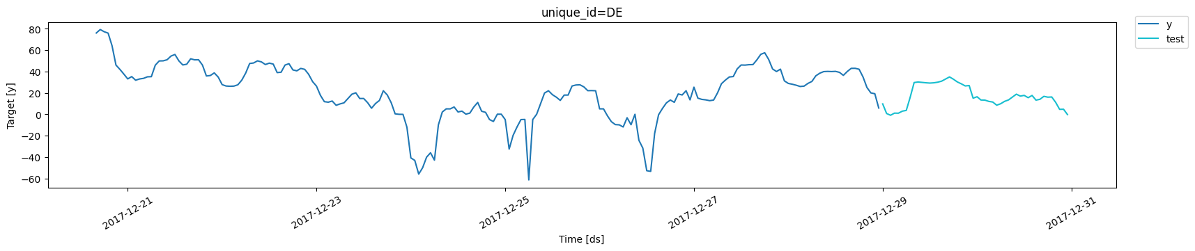

df = pd.read_csv('https://raw.githubusercontent.com/Nixtla/transfer-learning-time-series/main/datasets/electricity-short-with-ex-vars.csv')
df['ds'] = pd.to_datetime(df['ds'])
df_sub = df.query('unique_id == "DE"')

df_train = df_sub.query('ds < "2017-12-29"')
df_test = df_sub.query('ds >= "2017-12-29"')
df_train.shape, df_test.shape

((1632, 12), (48, 12))

plot_series(df_train[['unique_id','ds','y']][-200:], forecasts_df= df_test[['unique_id','ds','y']].rename(columns={'y': 'test'}))

2. Benchmark Forecasting using TimeGPT

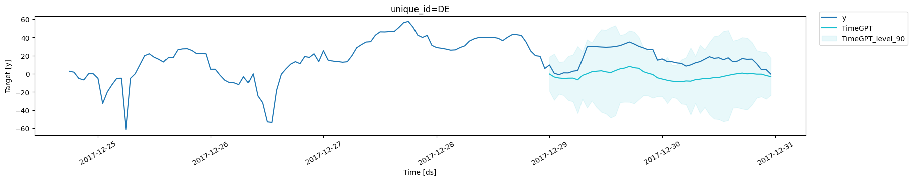
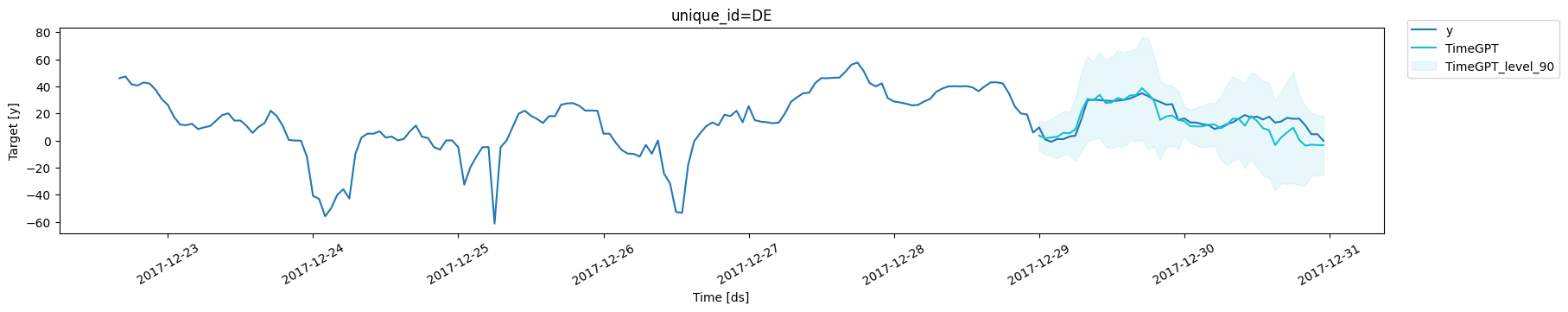
We used TimeGPT to generate a zero-shot forecast for the time series. As illustrated in the plot, TimeGPT captures the overall trend reasonably well, but it falls short in modeling the short-term fluctuations and cyclical patterns present in the actual data. During the test period, the model achieved a Mean Absolute Error (MAE) of 18.5 and a Root Mean Square Error (RMSE) of 20. This forecast serves as a baseline for further comparison and optimization.

fcst_timegpt = nixtla_client.forecast(df = df_train[['unique_id','ds','y']],
                                      h=2*24,
                                      target_col = 'y',
                                      level = [90, 95])

INFO:nixtla.nixtla_client:Validating inputs...
INFO:nixtla.nixtla_client:Inferred freq: h
INFO:nixtla.nixtla_client:Preprocessing dataframes...
INFO:nixtla.nixtla_client:Querying model metadata...
WARNING:nixtla.nixtla_client:The specified horizon "h" exceeds the model horizon, this may lead to less accurate forecasts. Please consider using a smaller horizon.
INFO:nixtla.nixtla_client:Restricting input...
INFO:nixtla.nixtla_client:Calling Forecast Endpoint...

metrics = [mae, rmse]

evaluation = evaluate(
    fcst_timegpt.merge(df_test, on=['unique_id', 'ds']),
    metrics=metrics,
    models=['TimeGPT']
)
evaluation

	unique_id	metric	TimeGPT
0	DE	mae	18.519004
1	DE	rmse	20.037751

plot_series(df_sub.iloc[-150:], forecasts_df= fcst_timegpt, level = [90])

3. Methods to Improve Forecast Accuracy

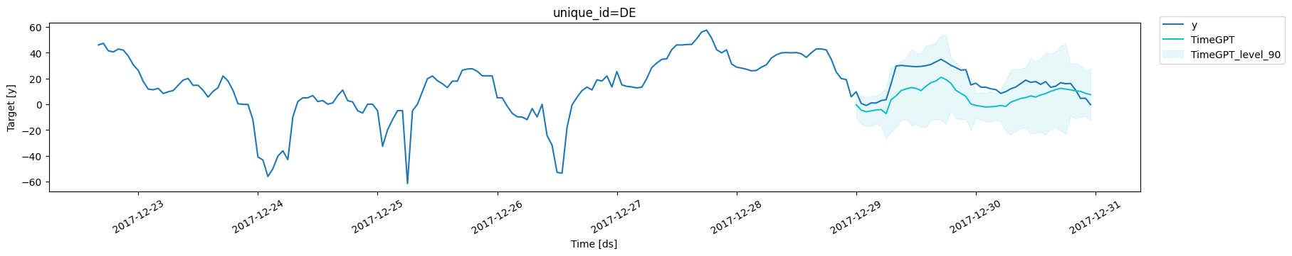
3a. Add Finetune Steps

The first approach to enhance forecast accuracy is to increase the number of fine-tuning steps. The fine-tuning process adjusts the weights within the TimeGPT model, allowing it to better fit your customized data. This adjustment enables TimeGPT to learn the nuances of your time series more effectively, leading to more accurate forecasts. With 30 fine-tuning steps, we observe that the MAE decreases to 11.5 and the RMSE drops to 12.6.

fcst_finetune_df = nixtla_client.forecast(df=df_train[['unique_id', 'ds', 'y']],
                                          h=24*2,
                                          finetune_steps = 30,
                                          level=[90, 95])

INFO:nixtla.nixtla_client:Validating inputs...
INFO:nixtla.nixtla_client:Inferred freq: h
INFO:nixtla.nixtla_client:Preprocessing dataframes...
WARNING:nixtla.nixtla_client:The specified horizon "h" exceeds the model horizon, this may lead to less accurate forecasts. Please consider using a smaller horizon.
INFO:nixtla.nixtla_client:Calling Forecast Endpoint...

evaluation = evaluate(
    fcst_finetune_df.merge(df_test, on=['unique_id', 'ds']),
    metrics=metrics,
    models=['TimeGPT']
)
evaluation

	unique_id	metric	TimeGPT
0	DE	mae	11.458185
1	DE	rmse	12.642999

plot_series(df_sub[-200:], forecasts_df= fcst_finetune_df, level = [90])

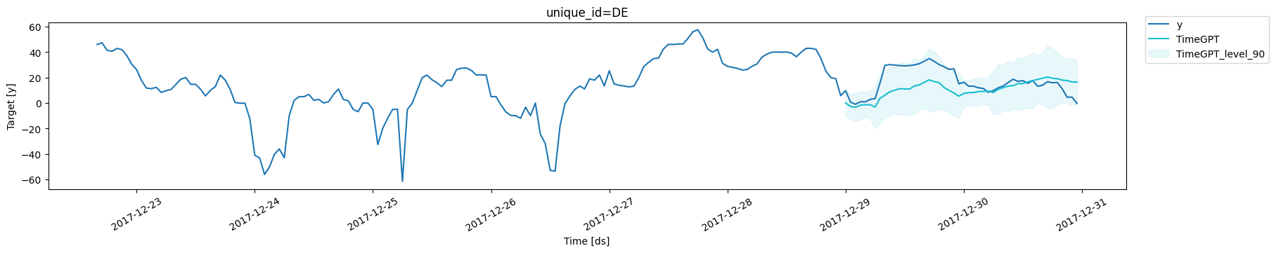
3b. Finetune with Different Loss Function

The second way to further reduce forecast error is to adjust the loss function used during fine-tuning. You can specify your customized loss function using the finetune_loss parameter. By modifying the loss function, we observe that the MAE decreases to 9.6 and the RMSE reduces to 11.0.

fcst_finetune_mae_df = nixtla_client.forecast(df=df_train[['unique_id', 'ds', 'y']],
                                          h=24*2,
                                          finetune_steps = 30,
                                          finetune_loss = 'mae',
                                          level=[90, 95])

INFO:nixtla.nixtla_client:Validating inputs...
INFO:nixtla.nixtla_client:Inferred freq: h
INFO:nixtla.nixtla_client:Preprocessing dataframes...
WARNING:nixtla.nixtla_client:The specified horizon "h" exceeds the model horizon, this may lead to less accurate forecasts. Please consider using a smaller horizon.
INFO:nixtla.nixtla_client:Calling Forecast Endpoint...

evaluation = evaluate(
    fcst_finetune_mae_df.merge(df_test, on=['unique_id', 'ds']),
    metrics=metrics,
    models=['TimeGPT']
)
evaluation

	unique_id	metric	TimeGPT
0	DE	mae	9.640649
1	DE	rmse	10.956003

plot_series(df_sub[-200:], forecasts_df= fcst_finetune_mae_df, level = [90])

3c. Adjust the number of parameters being fine-tuned

Using the finetune_depth parameter, we can control the number of parameters that get fine-tuned. By default, finetune_depth=1, meaning that few parameters are tuned. We can set it to any value from 1 to 5, where 5 means that we fine-tune all of the parameters of the model.

fcst_finetune_depth_df = nixtla_client.forecast(df=df_train[['unique_id', 'ds', 'y']],
                                                h=24*2,
                                                finetune_steps = 30,
                                                finetune_depth=2,
                                                finetune_loss = 'mae',
                                                level=[90, 95])

INFO:nixtla.nixtla_client:Validating inputs...
INFO:nixtla.nixtla_client:Inferred freq: h
INFO:nixtla.nixtla_client:Preprocessing dataframes...
WARNING:nixtla.nixtla_client:The specified horizon "h" exceeds the model horizon, this may lead to less accurate forecasts. Please consider using a smaller horizon.
INFO:nixtla.nixtla_client:Calling Forecast Endpoint...

evaluation = evaluate(
    fcst_finetune_depth_df.merge(df_test, on=['unique_id', 'ds']),
    metrics=metrics,
    models=['TimeGPT']
)
evaluation

	unique_id	metric	TimeGPT
0	DE	mae	9.002193
1	DE	rmse	11.348207

plot_series(df_sub[-200:], forecasts_df= fcst_finetune_depth_df, level = [90])

3d. Forecast with Exogenous Variables

Exogenous variables are external factors or predictors that are not part of the target time series but can influence its behavior. Incorporating these variables can provide the model with additional context, improving its ability to understand complex relationships and patterns in the data.

To use exogenous variables in TimeGPT, pair each point in your input time series with the corresponding external data. If you have future values available for these variables during the forecast period, include them using the X_df parameter. Otherwise, you can omit this parameter and still see improvements using only historical values. In the example below, we incorporate 8 historical exogenous variables along with their values during the test period, which reduces the MAE and RMSE to 4.6 and 6.4, respectively.

df_train.head()

	unique_id	ds	y	Exogenous1	Exogenous2	day_0	day_1	day_2	day_3	day_4	day_5	day_6
1680	DE	2017-10-22 00:00:00	19.10	16972.75	15778.92975	0.0	0.0	0.0	0.0	0.0	0.0	1.0
1681	DE	2017-10-22 01:00:00	19.03	16254.50	16664.20950	0.0	0.0	0.0	0.0	0.0	0.0	1.0
1682	DE	2017-10-22 02:00:00	16.90	15940.25	17728.74950	0.0	0.0	0.0	0.0	0.0	0.0	1.0
1683	DE	2017-10-22 03:00:00	12.98	15959.50	18578.13850	0.0	0.0	0.0	0.0	0.0	0.0	1.0
1684	DE	2017-10-22 04:00:00	9.24	16071.50	19389.16750	0.0	0.0	0.0	0.0	0.0	0.0	1.0

future_ex_vars_df = df_test.drop(columns = ['y'])
future_ex_vars_df.head()

	unique_id	ds	Exogenous1	Exogenous2	day_0	day_1	day_2	day_3	day_4	day_5	day_6
3312	DE	2017-12-29 00:00:00	17347.00	24577.92650	0.0	0.0	0.0	0.0	1.0	0.0	0.0
3313	DE	2017-12-29 01:00:00	16587.25	24554.31950	0.0	0.0	0.0	0.0	1.0	0.0	0.0
3314	DE	2017-12-29 02:00:00	16396.00	24651.45475	0.0	0.0	0.0	0.0	1.0	0.0	0.0
3315	DE	2017-12-29 03:00:00	16481.25	24666.04300	0.0	0.0	0.0	0.0	1.0	0.0	0.0
3316	DE	2017-12-29 04:00:00	16827.75	24403.33350	0.0	0.0	0.0	0.0	1.0	0.0	0.0

fcst_ex_vars_df = nixtla_client.forecast(df=df_train,
                                         X_df=future_ex_vars_df,
                                         h=24*2,
                                         level=[90, 95])

INFO:nixtla.nixtla_client:Validating inputs...
INFO:nixtla.nixtla_client:Inferred freq: h
INFO:nixtla.nixtla_client:Preprocessing dataframes...
WARNING:nixtla.nixtla_client:The specified horizon "h" exceeds the model horizon, this may lead to less accurate forecasts. Please consider using a smaller horizon.
INFO:nixtla.nixtla_client:Using future exogenous features: ['Exogenous1', 'Exogenous2', 'day_0', 'day_1', 'day_2', 'day_3', 'day_4', 'day_5', 'day_6']
INFO:nixtla.nixtla_client:Calling Forecast Endpoint...

evaluation = evaluate(
    fcst_ex_vars_df.merge(df_test, on=['unique_id', 'ds']),
    metrics=metrics,
    models=['TimeGPT']
)
evaluation

	unique_id	metric	TimeGPT
0	DE	mae	4.602594
1	DE	rmse	6.358831

plot_series(df_sub[-200:], forecasts_df= fcst_ex_vars_df, level = [90])

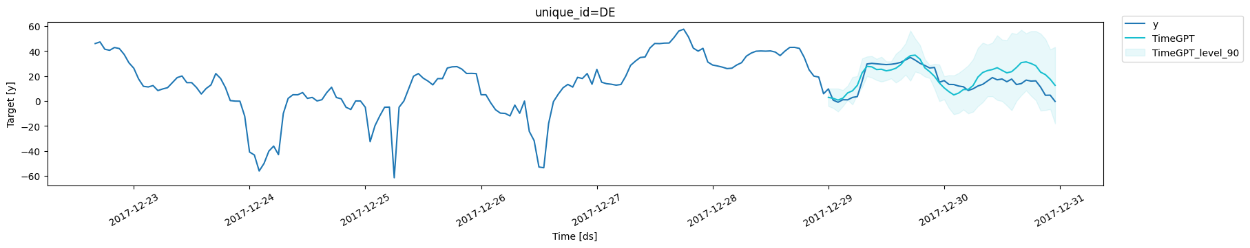
3d. TimeGPT for Long Horizon Forecasting

When the forecasting period is too long, the predicted results may not be as accurate. TimeGPT performs best with forecast periods that are shorter than one complete cycle of the time series. For longer forecast periods, switching to the timegpt-1-long-horizon model can yield better results. You can specify this model by using the model parameter.

In the electricity price time series used here, one cycle is 24 steps (representing one day). Since we’re forecasting two days (48 steps) into the future, using timegpt-1-long-horizon significantly improves the forecasting accuracy, reducing the MAE to 6.4 and RMSE to 7.7.

fcst_long_df = nixtla_client.forecast(df=df_train[['unique_id', 'ds', 'y']],
                                          h=24*2,
                                          model = 'timegpt-1-long-horizon',
                                          level=[90, 95])

INFO:nixtla.nixtla_client:Validating inputs...
INFO:nixtla.nixtla_client:Inferred freq: h
INFO:nixtla.nixtla_client:Preprocessing dataframes...
INFO:nixtla.nixtla_client:Querying model metadata...
INFO:nixtla.nixtla_client:Restricting input...
INFO:nixtla.nixtla_client:Calling Forecast Endpoint...

evaluation = evaluate(
    fcst_long_df.merge(df_test, on=['unique_id', 'ds']),
    metrics=metrics,
    models=['TimeGPT']
)
evaluation

	unique_id	metric	TimeGPT
0	DE	mae	6.365540
1	DE	rmse	7.738188

plot_series(df_sub[-200:], forecasts_df= fcst_long_df, level = [90])

4. Conclusion and Next Steps

In this notebook, we demonstrated four effective strategies for enhancing forecast accuracy with TimeGPT:

1. Increasing the number of fine-tuning steps.
2. Adjusting the fine-tuning loss function.
3. Incorporating exogenous variables.
4. Switching to the long-horizon model for extended forecasting periods.

We encourage you to experiment with these hyperparameters to identify the optimal settings that best suit your specific needs. Additionally, please refer to our documentation for further features, such as model explainability and more.

In the examples provided, after applying these methods, we observed significant improvements in forecast accuracy metrics, as summarized below.

Result Summary

Steps	Description	MAE	MAE Improvement (%)	RMSE	RMSE Improvement (%)
0	Zero-Shot TimeGPT	18.5	N/A	20.0	N/A
1	Add Fine-Tuning Steps	11.5	38%	12.6	37%
2	Adjust Fine-Tuning Loss	9.6	48%	11.0	45%
3	Fine-tune more parameters	9.0	51%	11.3	44%
4	Add Exogenous Variables	4.6	75%	6.4	68%
5	Switch to Long-Horizon Model	6.4	65%	7.7	62%